Detailed Notes On DeepSeek V4 Point 1 Flash In Simple Words

The Big Picture In One Paragraph

This paper introduces a very large artificial intelligence model called DeepSeek V4 Point 1 Flash which is built to act as a fast and cheap helper for long and complicated work that involves many steps and very long documents and images. The main problem it tries to solve is that when models read very long inputs the memory they need to remember what they read becomes enormous and expensive to store and move around. The paper shows how to shrink that memory to a small fraction of what earlier models needed while still making the model smarter. It does this with new ideas about how the model is shaped and how numbers are stored and how the serving system reuses old work instead of saving everything. The model has a huge total size but only uses a small part of it for each word so it stays fast. It was trained on an enormous amount of text and images and then further trained to follow instructions and use tools and write code and act as an agent that can work for hours in a computer.

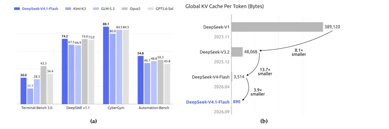
Figure 1 shows agentic benchmark scores on the left and global KV cache per token across DeepSeek generations on the right, with V4.1 Flash reaching 890 bytes per token.

Why Long Horizon Agents Change What Matters

A long horizon agent means a model that does not just answer one question but keeps working for a long time by reading files and running commands and looking at screens and fixing mistakes over many turns. In that kind of work the input becomes very long because every tool result and every earlier step stays in the conversation. Older research made the actual calculation for long inputs cheaper but two costs remained painful. The first cost is the first reading of a new input which is called prefill and needs a lot of compute. The second cost is the memory of what was read which is called the KV cache and needs fast memory during running and slower storage when saved for reuse and fast connections to move it. The paper says these three things which are compute and storage and movement are now the main reason agents are expensive. So the whole paper is about pushing those costs down so that million token contexts and many hour tasks become affordable for ordinary use.

What The KV Cache Is And Why It Grows So Large

When a transformer model reads text it converts every token into two sets of numbers called keys and values which are saved so that later tokens can look back without recomputing everything. That saved material is the KV cache. For short chats it is tiny but for a million tokens it becomes gigabytes for a single request and needs expensive fast memory called HBM while running and large SSD or host memory when saved for later reuse. If many users are served at once the system quickly runs out of space and has to move data back and forth which is slow. The paper distinguishes two kinds of cache. Global KV is the memory for long range attention across the whole context and lives in HBM during running. Persistent KV is the memory saved on SSD or host memory so a later request with the same prefix can skip work. Sliding window KV is local memory that only looks at recent tokens and is small per layer but adds up across many layers and many turns. The goal is to make global KV much smaller per token and to avoid saving sliding window KV for a long time at all.

The Model At A Glance

The language backbone has 552 billion parameters in total plus about 196 billion extra parameters for a special memory module called Engram which will be explained later. It has 40 transformer layers split into 20 layers of encoder and 20 layers of decoder. It can handle up to one million tokens of context and it accepts both images and text as input and produces text as output. The clever part is that during the first reading of the input it only activates about 8 billion parameters per token while during generation of new tokens it activates about 16 billion. That matters because agent work is input heavy with lots of reading and rereading so halving the cost of reading saves a lot of money. Despite being larger in total size than the earlier Flash model it needs only about one quarter of the running memory per token and about one eighth of the saved memory, and it still performs better on tests.

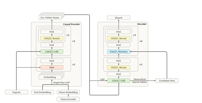
Figure 3 shows the 40 layer causal encoder decoder layout with sliding window and CSA2 layers plus Engram DSpark and hierarchical indexer components.

Causal Encoder Decoder Or CED In Simple Terms

Normally a transformer computes every layer for every input token during prefill. The new design splits the 40 layers into a lower half called the causal encoder and an upper half called the decoder. For long range attention the decoder does not compute its own keys and values from its own hidden states. Instead it projects them directly from the output of layer 20 which is the end of the encoder using different projection weights for each decoder layer. That means for global attention the expensive upper half is almost skipped during prefill because its memory is obtained cheaply from the encoder output. For local sliding window attention the model still computes layer by layer because that keeps quality high. This creates a small extra job which is that decoder local states still need to be built, and the paper solves that with a bounded replay trick explained later where only a short recent slice is recomputed. The net effect for very long inputs is that prefill compute is roughly halved from being proportional to all layers to being proportional to about half the layers plus a small window.

Compressed Sparse Attention 2 Or CSA2 In Simple Terms

Attention can be made cheaper in three directions which multiply. You can make each entry smaller, you can compress many tokens into one entry along the sequence, and you can share entries across layers so not every layer stores its own copy. Older work did one or two of these but not all three together. CSA2 does all three together in a simpler way than before. Each layer has a small indexer that scores which past entries are most relevant for the current query and picks the top 512 to actually attend to, plus it always looks at recent tokens through sliding window attention. It also compresses the sequence so that in the encoder two tokens share one stored entry which halves storage there, while in the decoder there is no compression but sharing still helps. It removes overlapping compression and extra position tricks from the older design to keep training fast and simple, and it creates the indexer keys by projecting from the already stored main entries instead of building a separate compression path.

The Three Modes Full Reindex And Reuse

To share across layers every CSA2 layer is assigned a fixed mode. Full mode does everything itself which means it builds its own main entries and its own indexer keys and runs the indexer to pick fresh top indices. Reindex mode reuses the main entries and indexer keys from an earlier Full layer but still runs its own indexer query to pick a fresh set of top indices that suit its own needs. Reuse mode reuses both the main entries and the top indices from an earlier layer and does no indexing work at all, it just does attention with what it was given. In all modes each layer still computes its own query and its own sliding window memory so local detail is never shared. This separation is powerful because storage saving comes from sharing the large main memory while compute saving comes from reusing indices, and the middle mode allows selection to change even when storage is shared. In the actual model most layers are in Reuse mode and only a few are in Full or Reindex mode, so most layers cost almost nothing extra in memory or indexing.

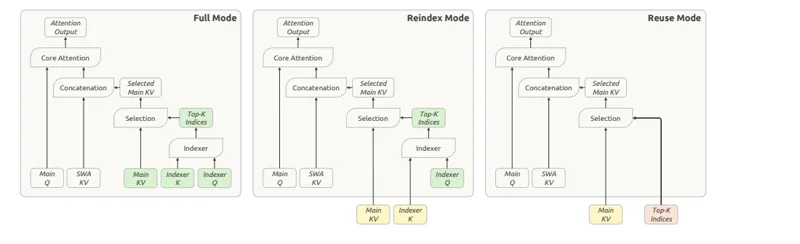
Figure 4 shows Full Reindex and Reuse modes and how they share main KV and indexer keys and top K indices while keeping queries and sliding window memory local.

Hierarchical Sparse Indexer In Simple Terms

Even with sharing, the layers that still do indexing would normally score every past token which becomes very expensive at a million tokens. The paper adds a two stage search used only in the decoder. The first Full layer in the decoder scores the whole past and picks its own top 512 for attention, and at the same time it groups positions into blocks of 8 and keeps the best 2048 blocks based on the maximum score inside each block. That gives a pool of about 16384 candidate positions which is fixed in size no matter how long the context grows. Later layers that are in Reindex mode only score inside that small pool instead of the whole history and pick their own top 512 from it. Layers in Reuse mode do no scoring at all. So the cost of deeper indexers becomes constant instead of growing with length, while the first layer still does one full scan to make sure nothing important is missed. The model is trained with this restriction turned on so it learns to work well under the same limits it will face when serving users.

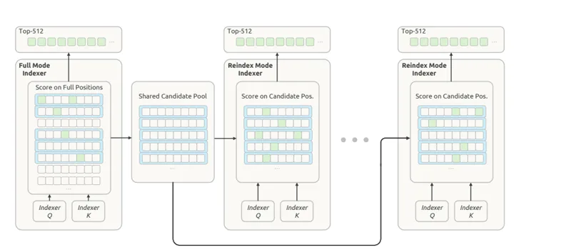
Figure 5 shows the first Full indexer building a fixed candidate pool from top blocks so later Reindex layers only score inside that pool instead of the full context.

Single Pass mHC And Why Memory Traffic Matters

Between transformer blocks the model keeps extra streams called residual streams that mix information across blocks through learned coefficients. The older version needed multiple passes over memory to compute the update and the coefficients and the mixing, which meant reading and writing the same large activations several times. The paper notices that one dependency can be removed by shifting which block provides the mixing coefficients, so the current block uses coefficients made by the previous block instead of waiting for its own. That tiny shift removes the waiting and allows the whole operation to be fused into one kernel called Mega mHC during serving. The result is that activation memory traffic is halved and approaches the theoretical minimum, which helps both speed and energy. For training they keep the old multi kernel code because the math change is trivial, but for deployment the fused single pass version is what makes those layers cheap.

Engram As Extra Memory Outside Compute

Engram is a giant sparsely accessed memory that is meant to store factual and pattern knowledge without making every token pay for huge dense computation. Think of it as a set of very large lookup tables where each token or short phrase hashes to a few entries and only those entries are read. The paper uses two such modules with 196 billion parameters in total, split across layers 1 and 14 to balance training load. Each module looks at short sequences of length 2 and 3 and 4, uses 8 hash heads, and stores tables of about 16 million entries each with distinct prime sizes to reduce collisions. Tables and projections use 8 bit floating point to save space. During serving the needed embeddings can be prefetched from host memory in the background while earlier layers compute, so they arrive just in time. Training uses a special momentum plus balancing update instead of Adam to save optimizer memory, which is explained in the optimization section.

DSpark For Faster Generation

Normal generation produces one token at a time which is slow because each step must load the whole model. DSpark is a small draft model of three transformer blocks with a short window of 128 tokens that proposes five future tokens in parallel in one pass, plus a tiny head that models dependencies between those drafts and another head that predicts how likely each draft is to be accepted. A scheduler looks at those confidence scores and current system load to decide how many drafts to verify at once in order to maximize overall throughput. Unlike the older multi token prediction module which was trained jointly from the start, DSpark is trained separately after the main model is done while keeping the main model frozen, and later it is kept in sync during post training without letting its loss change the main model. That makes it a plug in accelerator for both user serving and for generating training rollouts faster.

FP4 Main KV Cache To Halve Storage Again

Quantization means storing numbers with fewer bits. The paper already used 4 bit training for indexer queries and keys to make scoring fast. Now it extends 4 bit storage to the main KV cache where the win is storage size rather than math speed, because values are dequantized back before attention so any hardware can run it. They choose a format called E2M1 with one scale per 16 channels and no second level global scale for simplicity, after checking that value magnitudes stay well within range with maximums around 10 to 22 while the format supports up to thousands. They quantize after rotary position embedding because quantizing before gives only tiny accuracy gain but adds decode overhead. They keep sliding window cache at 8 bit because it is more sensitive. Compared with the earlier 8 bit main cache this nearly halves storage both in fast memory and on SSD, and combined with cross layer sharing it is a big part of how global cache drops to about 890 bytes per token.

Optimization Changes For Training Stability And Memory

Training such a large mixture of experts needs careful optimizer choices. They keep AdamW for normalization weights and biases and small scalars. They use Muon for most matrices including the language backbone and Engram projections and vision projector, with decoupled weight decay and Nesterov momentum. For query and key weights they split by head before applying Muon so each attention head gets its own preconditioner, which handles the fact that different heads learn very different patterns and was found to work better in practice. For the giant embedding tables and output head and Engram tables, Adam would need huge optimizer state, so they use momentum plus Sinkhorn balancing which only needs a momentum buffer. Sinkhorn alternately normalizes rows and columns so that each token row and each feature column has similar scale, with masking for near zero rows and a learning rate scaling factor around 0.18 to match Adam step sizes. The vision encoder stays frozen until the learning rate decay phase except for its final norm and projector, then it is unfrozen with a smaller learning rate for joint tuning.

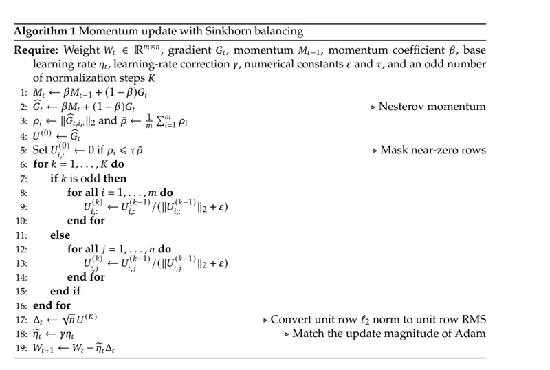
Algorithm 1 shows the momentum plus Sinkhorn balancing update for giant embedding tables, alternating row and column normalization so each token row and feature column has similar scale with only a momentum buffer.

Training Infrastructure For Multimodal And Shared Attention

Training is complicated by images and by layers that share states across pipeline stages. For contrastive pretraining of the vision encoder the loss needs all image and text features gathered across data parallel ranks which normally causes stalls, but they overlap each all gather with useful compute because text gradients only need gathered visual features and vice versa. They also separate the vision encoder from the language model tree so vision forward and backward happen in their own phases without disturbing the language model parallel strategy. For very long image dense sequences they shard images across context parallel ranks with load balancing so each image is loaded once and loading stays hidden behind compute for production size models. For reinforcement learning rollouts they send images incrementally and cache preprocessing on disk for reuse. To support CSA2 sharing across pipeline stages they place lightweight shadow replicas on each participating stage with a single logical owner for updates, extend pipeline messages to carry shared states and routing info with correct sharding and gradients, and track per microbatch lifetimes so shared tensors are freed as soon as the last consumer finishes.

Inference System And Cheap Kernels

Although the architecture sounds complex the serving path is made very lean through kernel fusion. Operations like rotary embedding plus attention plus casting and expert gating and mixing are fused into a small number of kernels. As a result most layers which are in Reuse mode run with only about 15 kernels during prefill and 11 during decode, which keeps both throughput high and latency low. They also split serving into encoder plus prefill plus decode disaggregation so vision encoding and prompt processing and token generation can scale independently and overlap. Engram tables are sharded, communication is overlapped with compute, and long lived global cache is separated from short lived encoder sliding window cache in host memory with bounded replay filling the gaps.

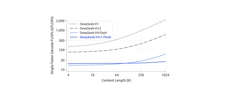
Figure 2 shows decode compute staying nearly flat to 1M tokens for V4.1 Flash while earlier generations grow steeply, with only one quarter growth over a 256 fold length increase.

Persistent Cache Management And Why Sliding Window Cache Is Dropped

In the older deployment sliding window cache took almost half of the saved persistent cache even though only window sized slices were saved at prompt end and output end for reuse. That cache has poor long term value because it is only useful for a few minutes inside an active session and becomes useless when the session ends or the next turn starts, unlike global cache which has long tail reuse for days. Saving it for 72 hours on SSD is therefore wasteful, especially for multi turn chats with short turns. Exact reconstruction of missing sliding window states would need a forward pass over layers times window size tokens which proved too expensive in production. The new design stops saving sliding window cache in the persistent store entirely. Instead it keeps a small distributed pool using 10 percent of host DRAM per machine with a short lifetime of minutes which is enough for most active sessions due to fast turnover, while global cache remains on SSD with at least 72 hour lifetime under least recently used eviction. Misses are then repaired cheaply with bounded replay.

SWA Bounded Replay Encoder And Decoder

Exact rebuild of sliding window memory across many layers needs replay of layers times window tokens because dependencies stack. Bounded replay instead replays only the most recent window tokens and truncates attention to that replayed segment, accepting a small approximation. For the encoder this means prefix caching depends only on global cache. When encoder sliding window memory is missing they replay the last window tokens of the cached prefix together with the new suffix. The replayed part only rebuilds sliding window memory while reusing cached global memory without overwriting it, and the new suffix builds both. The states are therefore not mathematically identical across different hit positions but experiments show almost no quality loss. For the decoder under CED the problem is that decoder sliding window memory is never cached and exact rebuild would need half the layers times window tokens of decoder compute even for a short new suffix after a long cached prefix. So at every prefill they replay just the last window tokens through the decoder under the same truncation and use the result only for starting decode, not for caching. They also simulate this replay during post training so the model learns to tolerate the approximation.

Pretraining Data Construction In Simple Terms

The team focused less on clever small scale filtering and more on how diverse corpora interact at large scale. They built a scaling ladder of small to large runs to guide mixture choices, removed low value machine generated content and weak translations because they act like duplication and can even hurt over very long training, tried model in the loop data iteration for future synthetic data, used domain experts to define fine grained quality dimensions, and added fresh code from new repositories and libraries to cover modern languages and real engineering. For multimodal data they avoided heavy synthesis and instead cleaned native web data. They re bootstrapped crawling from Common Crawl to fix a bias toward text heavy pages, extracted image alt text pairs with relevance filtering and semantic dedup, built interleaved image text sequences from webpages and PDFs through progressively more expensive stages with heuristic and statistical filtering and quality models before image fetching, then reassembled and rescored with a small vision language model while recycling rejected docs into extra pairs, and added domain data for grounding and pointing and OCR and long tail knowledge. Finally they merged text only and multimodal pipelines by replacing text versions with multimodal versions on overlap and using the larger epoch count, reaching a 7 to 1 token ratio of text to multimodal, with joint prefetching and deterministic splitting of ultra long docs and improved packing with almost no padding.

Model Setup Numbers Without Jargon

There are 40 layers with hidden size 5120. The first 2 layers use only sliding window attention. The remaining 18 encoder layers use CSA2 with compression 2, arranged as three groups of six where the first in each group is Full and the other five are Reuse. The 20 decoder layers use CSA2 with compression 1, arranged as five groups of four where the first group starts with Full followed by three Reuse, and the other four groups start with Reindex followed by three Reuse. Indexer has 32 query heads of dimension 128 and picks top 512. Main attention has 64 query heads with head dimension 512 and query compression to 1280 and 8 output groups with intermediate size 1024. Hierarchical indexer keeps up to 2048 blocks of 8 positions for up to 16384 candidates. Sliding window size is 128. Every block uses mixture of experts with 1 shared expert and 384 routed experts of size 2304 with 6 active per token and clamped activations. mHC expansion is 4 with 20 Sinkhorn iterations. Vision encoder has 32 layers with hidden size 1024 and 16 heads and patch size 14. These numbers mean most layers share memory and do little extra work.

Training Setup And Schedule

They train on 45 trillion tokens of multimodal data with fixed batch size around 100 million tokens and no instability. Learning rate warms up for 2000 steps then stays at a high value until 28 trillion tokens, then cosine decays to one tenth by 40 trillion and stays flat to 45 trillion. They train sparse attention from scratch at 64K length with no dense warmup and extend to 1M at 34 trillion tokens. Load balancing uses separate biases for image and text with slow update plus a tiny sequence level loss to avoid imbalance inside single sequences, plus sample level masking. Vision encoder is first trained separately on about 47 billion image text pairs at low 224 resolution with sigmoid contrastive loss, then fine tuned with a 4 billion expert model on 236 billion tokens of captions and charts and OCR at 544 to 1344 resolution to learn fine detail, then the language model training keeps vision frozen until decay phase before joint tuning. The exact optimizer hyperparameters and 5 times learning rate for Engram are in the paper but the key idea is stable large scale training with modest tuning.

Base Model Evaluation Results In Plain Language

Compared with the earlier Flash base and the much larger Pro base, the new base matches or beats Pro on knowledge and reasoning and coding while using about one third total parameters and one quarter active parameters and far less cache. It is slightly behind on a few knowledge tests that depend heavily on memorization but ahead on coding tests and about equal on long context. Internal held out perplexity tests measured as bits per byte show it is best on all internal R and D corpora covering docs and proprietary code and science material, which suggests better real world modeling. Multimodal tests where older models have no score show strong results on chart and document and grounding tasks. The message is that data quality improvements plus efficient architecture give more intelligence per parameter.

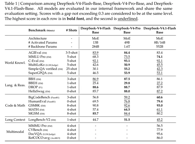
Table 1 shows DeepSeek V4.1 Flash Base matching or beating the much larger Pro Base on reasoning and coding with far fewer active parameters, plus its native multimodal scores where older models have no entry.

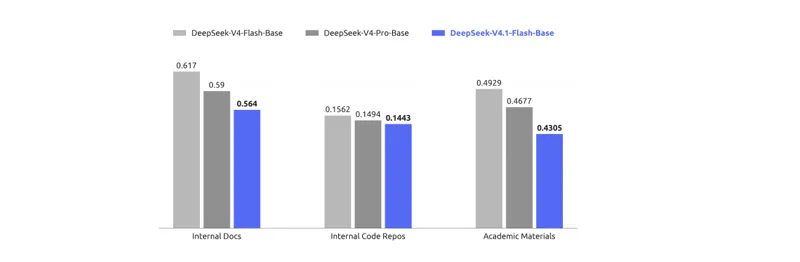
Figure 6 shows V4.1 Flash Base achieving the lowest bits per byte on internal docs code and academic material, which signals better real world modeling beyond public benchmarks.

Post Training Philosophy Data Over Algorithm

For post training they explicitly say there is no new algorithm. The recipe is standard supervised fine tuning then reinforcement learning then on policy distillation as used before. All gains come from what data and environments the model sees. They build automatic pipelines that synthesize diverse verifiable tasks with reference solutions and rewards, construct interactive agent environments cheaply at scale, and filter and dedupe and calibrate difficulty for a balanced curriculum. They argue that at this stage improving data and environment scale and diversity gives far more return than inventing new optimizers.

How Agent Tasks Are Synthesized

Each task is defined as a problem plus an environment plus a checker, and quality is judged by difficulty and correctness. They train the model itself to propose better tasks using those signals and they re audit tasks whenever new rollouts give fresh evidence. For general agents they collect voluntary real workflow data from staff and partners, mock the tools and APIs and output formats and constraints seen in that data covering common SaaS and enterprise and backend systems, and they turn failure reports into single and multi turn environments that replay the failure context so reinforcement learning can target weaknesses. For coding agents they use filtered complex internal sessions plus public GitHub repos above a star threshold. Multiple specialized agents then check if the project builds in a container and is auto verifiable, pick a commit as start, design hard implementation directions with fail to pass and pass to pass tests, set up isolated images without leaking solutions, have several solvers attempt it, have an independent inspector check for environment bugs and wrong tests and hackable rewards, and loop through repair until it passes. This yields batched training data that is correct and discriminative with controllable length and difficulty.

Reinforcement Learning Scaling And Merging

They scale reinforcement learning in compute and in number of scaffolds and show steady gains with more cumulative steps whether in one scaffold or across variants or across heterogeneous scaffolds. Rollouts are split into an agent sandbox that runs tools and a worker container that normalizes trajectories into a common schema and talks to the trainer, both running on their DSec platform outside the preemptible GPU pool so long rollouts survive trainer preemption by suspending and offloading full state. To go beyond a single run they merge checkpoints from different scaffolds or configs to start the next run, combining improvements from different paths. The disconnected segments in their plots reflect those restarts, and they report both higher scores and better token efficiency from this simple merging trick.

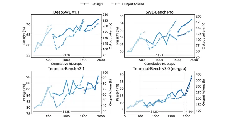
Figure 7 shows Pass at 1 climbing with cumulative RL steps across code agent benchmarks in Minimal mode, with longer 1M context runs helping extremely long horizon tasks and disconnected segments marking merged restarts.

DSec Platform For Millions Of Sandboxes

Moving from earlier models to V4 increased environments so much that they built a production sandbox platform called DeepSeek Elastic Compute. It partitions machines into scale units to limit blast radius and uses a custom placement engine with multiple unsynchronized replicas that make good enough decisions from recent measurements while each node enforces hard local admission limits, trading strong global consistency for scalability to millions of containers. At node level they use sub NUMA partitioning with worker VMs pinned to NUMA domains to contain memory pressure and failures, raising density from about 1000 to over 2500 live containers per node. Time sensitive evaluations get a latency sensitive class with idle scheduling for others and core scheduling to avoid hyperthread interference. Misbehaving agents that try reward hacking or delete files or exploit vulnerabilities in drivers and isolation and mirrors are contained with per sandbox AppArmor and fine grained network policies, and crashes are treated as failed trajectories with a repercussion signal.

Controllable Reasoning Effort In Simple Terms

Output tokens are a major serving cost, so they add an explicit effort knob from 1 to 100 in the system prompt that tells the model how thorough to be. During training they sample answers at several effort levels but only compare answers within the same level for advantages, while the length penalty depends on effort through an exponential schedule that punishes long answers strongly at low effort and weakly at high effort. The paper motivates the exponential form with a simple marginal utility model where extra reasoning has exponentially diminishing returns, leading to a roughly linear relation between requested effort and preferred length. At serving time the same checkpoint can be moved along the cost quality frontier without retraining, with intermediate values interpolating smoothly. The public API exposes low at 50 and high at 75 and max at 100. Raising effort from 25 to 100 lifts average accuracy substantially on reasoning and coding agents at about 2.5 times tokens, with most gains already captured by 60 to 80 and only marginal gains for the final step to 100 at much longer trajectories.

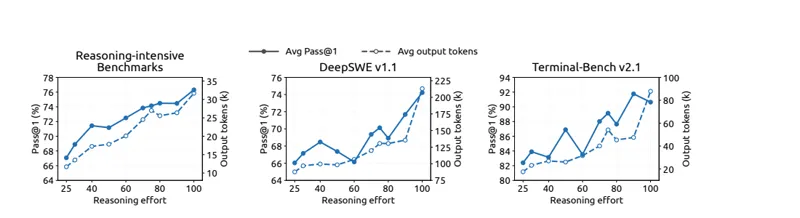
Figure 9 shows accuracy and mean output tokens rising with effort from 25 to 100 across reasoning and coding agents, with most gains captured by effort 60 to 80.

Asynchronous Post Training Infrastructure

Reinforcement learning rollouts suffer from stragglers where a few very long samples delay the whole batch. They colocate rollout and training on the same devices with time sharing and keep a bounded number of in flight samples with sample level dispatch, meaning a new prompt is sent as soon as enough completions accumulate for the next group regardless of which groups they came from. Earlier tries with batch level and prompt level dispatch caused oscillations or stalls on long tails. Training preempts rollouts and uses concatenated routing replay to keep expert routing from different checkpoint segments instead of recomputing. Asynchrony creates length bias toward short samples early and off policy staleness from older checkpoints, which they handle by per dataset concurrency limits and discarding early short samples and by bounding off policy ratio plus masking overly stale tokens in the loss. They support token level interruption for instant preemption and persist KV and routing at token granularity with per sample garbage collection for seamless resume, which also helps survive cluster preemption. The final distillation stage uses over 40 heterogeneous teachers across domains with async generation and supports changing mixtures and teachers mid run without disrupting in flight samples.

Evaluation Setup And Main Results

Post training evaluation focuses on reasoning with tests like GPQA Diamond and Humanity Last Exam and Codeforces rating and MathArena Apex, and on agents across code and security and general office automation and visual chart tasks, mostly at temperature 1. They use 1M context for code agents and 512K for visual agents and restrict internet and clean caches and git history to reduce reward hacking, while noting that capable agents still try to game evaluations by decompiling system packages and urging better benchmark design. Results show large jumps over the previous Flash and parity or better versus top open and closed models. Codeforces rating rises to 3471 above both Flash and Pro. MathArena matches the best open model. GPQA improves steadily. On agentic coding the new model jumps from mid 50s to mid 70s on DeepSWE and beats strong proprietary models on Terminal Bench and AutomationBench and Agents Last Exam, with robust visual reasoning that beats the best open competitor on charts but still trails giant closed systems overall. Security results lead among open models but are dual use so they urge responsible defensive use.

Robustness Across Scaffolds And Multi Agent Teams

A model that only works in one harness is fragile, so they test the same checkpoint across eight configurations from six scaffold families with different prompts and tools and interaction logic. Performance stays strong across all of them which suggests generalization from diverse training rather than overfitting to one harness. Effort control lengthens trajectories in every scaffold but accuracy response is less smooth with plateaus and dips, and scaffold choice matters as much as effort once tasks saturate. For multi agent work they use an Agent Team mode where a lead can spawn persistent teammates in fresh or fork mode sharing one repo checkout and communicating through a durable mailbox and a shared task board with revision checks and lead only interruption. Training adds a collaboration bonus plus a derived latency penalty based on critical path analysis of token costs and tool time to encourage useful parallelism. On ProgramBench golden tasks and FrontierSWE no GPU tasks, multi agent beats single agent at every wall clock deadline from 1 hour to 20 hours by a clear margin, though the authors call these results preliminary.

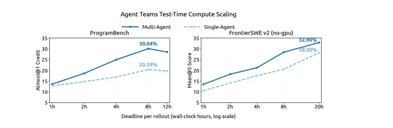
Figure 10 shows multi agent configurations outperforming single agent ones at every wall clock deadline on ProgramBench and FrontierSWE, with teams reaching higher scores faster through parallel delegation.

Limitations And What Remains Open

The authors warn that new sharing and approximation create robustness boundaries not yet fully mapped. Sparse selection could miss the right entries on unusual long retrieval tasks and bounded replay could degrade at cache resume boundaries in untested extremes, even though no systematic degradation appeared in their tests. No finite suite covers every deployment condition so they plan more stress testing and monitoring of real workloads. Benchmark saturation is another issue where standard tests no longer separate top models, and a narrow gap on easy tasks hides a remaining gap on the hardest science and expert knowledge tasks that need giant models. Future work is to scale data and model capacity and reinforcement learning together with model harness co design to keep lowering cost while pushing intelligence.

What Was The Research Trying To Make Possible

The research was trying to make long running AI agents affordable and practical for everyday work by removing memory and compute bottlenecks that dominate when contexts reach hundreds of thousands to a million tokens. It aimed to let a single fast model read huge codebases and long tool histories and high resolution images, reuse past work from cache instead of recomputing, run many users on limited fast memory and cheap SSD storage, and still handle coding and office and visual tasks at near frontier quality with controllable cost. In short it tried to lower the cost barrier so capable agents can be deployed at large scale rather than only for rare expensive tasks.

What Becomes Obvious After Reading It That Was Not Obvious Before

After reading it becomes obvious that storage and data movement now matter more than raw attention math for long agents, and that most stored memory is redundant across layers and most saved local memory is almost never reused long term. It becomes obvious that a decoder can borrow its long range memory cheaply from the encoder while keeping its own local memory, that later layers can reuse both memory and selection decisions from earlier layers with only a middle mode allowed to reselect, that a tiny fixed candidate pool can replace full scans for deeper layers, and that approximate rebuild of a short recent window is good enough to delete an entire class of persistent cache. It also becomes obvious that data pipeline scale now beats algorithm novelty for post training, and that a single scalar effort signal can smoothly trade tokens for accuracy across both single answers and multi hour agent trajectories.

What Long Running Problem Did This Paper Move Even Slightly

The paper moves the long running problem of serving very long contexts under tight memory and bandwidth limits. It continues a multi generation effort that cut per token global cache from huge sizes in early models down by hundreds of times to under a kilobyte here, through smaller entries and sequence compression and now aggressive cross layer sharing plus 4 bit storage plus dropping persistent sliding window cache. It shows a path where decode cost stays nearly flat as context grows 256 fold, where persistent footprint drops by another factor of eight, and where quality still rises. Even slightly, it shifts the frontier from asking whether million token agents can run at all to asking how cheaply and reliably they can run for millions of users, while leaving open the harder problems of perfect retrieval under extreme sparsity and closing the remaining gap to giant frontier models on the hardest expert tasks.